Statistical Arbitrage: Difference between revisions
No edit summary |
No edit summary |
||
| Line 1: | Line 1: | ||
'''Statistical Arbitrage Strategy''' relies on the historically strong correlation between two financial instruments, for example, WTI and Brent, DE30 and F40, Amazon and Apple. Users can set a period for correlation determination, timeframe, and strong correlation level. The software sells strong and buys weak instruments when their correlation diverges beyond a certain level. Once mean reversion occurs, the locked position created by the two orders: buy and sell, should generally be in profit. This strategy is also known as convergence or pair trading. | |||
'''THE CORE PRINCIPLE''' | |||
Statistical arbitrage relies | Statistical arbitrage relies on mean reversion principles and the law of large numbers. The underlying belief is that the relative prices of financial instruments that are historically correlated will revert to their mean over time. This is where statistical arbitrage occurs – it capitalizes on price discrepancies between these correlated instruments when they deviate from their historical norm. | ||
For instance, consider two stocks that have moved together historically. If their prices diverge – one increases in price, and the other decreases – a statistical arbitrageur would sell short the outperforming stock and buy the underperforming one, betting that the “spread” between the two would eventually converge. | |||
'''SPREAD – TO THE PRICE DIFFERENCE OR DISCREPANCY BETWEEN TWO RELATED FINANCIAL INSTRUMENTS.''' | |||
In statistical arbitrage, the term ‘spread’ typically refers to the price difference or discrepancy between two related financial instruments. These could be two different stocks, futures contracts, forex pairs, or even cryptocurrency tokens. | |||
For example, one might track the spread between two historically co-integrated stocks in a pair trading strategy (a common form of statistical arbitrage). When the spread, or the difference in their prices, deviates significantly from its historical mean (average), it signals an opportunity to trade. | |||
Suppose the spread widens too much, indicating one stock is overpriced and the other is underpriced relative to their historical relationship. In that case, a trader may sell short the overpriced stock and buy the underpriced one. Conversely, if the spread narrows excessively, they would do the opposite. | |||
The spread is expected to be mean-reverting in statistical arbitrage, meaning it fluctuates around a long-term average value. Traders expect that when the spread deviates significantly from this mean, it will eventually return to it, allowing them to profit from this reversion. | |||
[[File:Sl.png|center|frameless|927x927px]] | |||
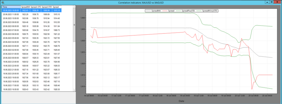
In the SharpTrader platform Spread Indicator is used to visualize the correlation between two assets. The calculation of the correlation involves the following components: | |||
* Spread: This refers to the numerical difference or distance between the values of two assets. | |||
* SpreadMA: It represents the moving average of the spread over a specific period, determined by pi_SpreadMA_Period. | |||
* STD (Standard Deviation): It calculates the classic standard deviation of the spread relative to SpreadMA. The number of observations used is equal to pi_SpreadMA_Period. | |||
To trigger the opening of trades, the software follows the principles of statistical arbitrage theory. | |||
[[File:Sl2.png|center|frameless|469x469px]] | |||
''' | === '''STATISTICAL ARBITRAGE – CORRELATION MATRIX''' === | ||
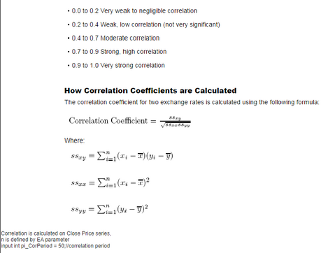
A correlation table, also known as a correlation matrix, is a table that shows the correlation coefficients between many variables. Each cell in the table shows the correlation between two variables. The value is in the range of -1 to 1. | |||
If two variables have a correlation of 1, they move in the same direction, i.e., when one increases, the other increases, and vice versa. This is known as a perfect positive correlation. | |||
If two variables correlate -1, they move in opposite directions, i.e., when one variable increases, the other decreases, and vice versa. This is known as a perfect negative correlation. A correlation of 0 means that no relationship exists between the variables. | |||
Here’s a simple example of a correlation table for three variables: A, B, and C: | |||
[[File:Sl3.png|center|frameless|515x515px]] | |||
In this table, the correlation between variables A and B is 0.5 (a moderate positive correlation), while the correlation between A and C is -0.7 (a strong negative correlation). The diagonal of the matrix from the top left to the bottom right is always 1 because a variable is perfectly correlated with itself. | |||
These tables are widely used in various fields, including finance, where they help in determining the relationship between different financial variables or the returns of different assets, useful for portfolio diversification and risk management. | |||
Revision as of 18:15, 4 September 2023
Statistical Arbitrage Strategy relies on the historically strong correlation between two financial instruments, for example, WTI and Brent, DE30 and F40, Amazon and Apple. Users can set a period for correlation determination, timeframe, and strong correlation level. The software sells strong and buys weak instruments when their correlation diverges beyond a certain level. Once mean reversion occurs, the locked position created by the two orders: buy and sell, should generally be in profit. This strategy is also known as convergence or pair trading.
THE CORE PRINCIPLE
Statistical arbitrage relies on mean reversion principles and the law of large numbers. The underlying belief is that the relative prices of financial instruments that are historically correlated will revert to their mean over time. This is where statistical arbitrage occurs – it capitalizes on price discrepancies between these correlated instruments when they deviate from their historical norm.
For instance, consider two stocks that have moved together historically. If their prices diverge – one increases in price, and the other decreases – a statistical arbitrageur would sell short the outperforming stock and buy the underperforming one, betting that the “spread” between the two would eventually converge.
SPREAD – TO THE PRICE DIFFERENCE OR DISCREPANCY BETWEEN TWO RELATED FINANCIAL INSTRUMENTS.
In statistical arbitrage, the term ‘spread’ typically refers to the price difference or discrepancy between two related financial instruments. These could be two different stocks, futures contracts, forex pairs, or even cryptocurrency tokens.
For example, one might track the spread between two historically co-integrated stocks in a pair trading strategy (a common form of statistical arbitrage). When the spread, or the difference in their prices, deviates significantly from its historical mean (average), it signals an opportunity to trade.
Suppose the spread widens too much, indicating one stock is overpriced and the other is underpriced relative to their historical relationship. In that case, a trader may sell short the overpriced stock and buy the underpriced one. Conversely, if the spread narrows excessively, they would do the opposite.
The spread is expected to be mean-reverting in statistical arbitrage, meaning it fluctuates around a long-term average value. Traders expect that when the spread deviates significantly from this mean, it will eventually return to it, allowing them to profit from this reversion.

In the SharpTrader platform Spread Indicator is used to visualize the correlation between two assets. The calculation of the correlation involves the following components:
- Spread: This refers to the numerical difference or distance between the values of two assets.
- SpreadMA: It represents the moving average of the spread over a specific period, determined by pi_SpreadMA_Period.
- STD (Standard Deviation): It calculates the classic standard deviation of the spread relative to SpreadMA. The number of observations used is equal to pi_SpreadMA_Period.
To trigger the opening of trades, the software follows the principles of statistical arbitrage theory.

STATISTICAL ARBITRAGE – CORRELATION MATRIX
A correlation table, also known as a correlation matrix, is a table that shows the correlation coefficients between many variables. Each cell in the table shows the correlation between two variables. The value is in the range of -1 to 1.
If two variables have a correlation of 1, they move in the same direction, i.e., when one increases, the other increases, and vice versa. This is known as a perfect positive correlation.
If two variables correlate -1, they move in opposite directions, i.e., when one variable increases, the other decreases, and vice versa. This is known as a perfect negative correlation. A correlation of 0 means that no relationship exists between the variables.
Here’s a simple example of a correlation table for three variables: A, B, and C:

In this table, the correlation between variables A and B is 0.5 (a moderate positive correlation), while the correlation between A and C is -0.7 (a strong negative correlation). The diagonal of the matrix from the top left to the bottom right is always 1 because a variable is perfectly correlated with itself.
These tables are widely used in various fields, including finance, where they help in determining the relationship between different financial variables or the returns of different assets, useful for portfolio diversification and risk management.